Sandia validation case

The hydrogen-forklift release experiments by Ekoto, Houf, Evans, Merilo and Groethe [1, 2] were a series of tests aimed at improving the understanding of hydrogen releases, dispersion, accumulation and ignition behaviour relating to fuel-cell powered forklifts operating in enclosed spaces. The objective was to develop an experimental dataset that could be used to validate dispersion and ignition models, assess hazard mitigation and support the integration of hydrogen-powered vehicles indoors in spaces like warehouses.

The work focused on:

• Generation of experimental data for hydrogen releases from forklift fuel-cell systems within confined or semi-confined indoor geometries.

• Investigation of the interaction between hydrogen jet/plume behaviour and warehouse ventilation, including natural stratification and accumulation beneath ceilings.

• Assessment of explosions following ignition, including flame progression and pressure development.

The programme was carried out at Sandia National Laboratories with participation from the U.S. Department of Energy and industrial partners involved in hydrogen fuel-cell vehicle deployment.

The outcome of the work was experimental data relating to hydrogen leak rates, dispersion profiles, flammable cloud formation, ignition outcomes and overpressure measurement that could be used to validate modelling approaches.

Experimental setup

The experiments were conducted in a subscale test facility representing a warehouse environment in which hydrogen fuel-cell forklifts could operate.

A series of releases was conducted within enclosed or semi-enclosed test compartments, with a variety of ventilation arrangements including no ventilation, forced ventilation or natural ventilation.

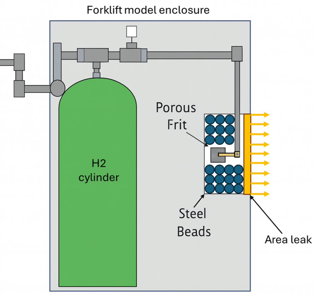
Hydrogen was released from a model of a forklift, consisting of a cuboidal enclosure containing a modified hydrogen cylinder. The release exited the enclosure via a packed area of steel beads fitted with a porous frit which would allow hydrogen to exit in a uniform manner.

The tank specification for the subscale model was as follows:

• Tank pressure = 134.5 bar

• Tank volume = 3.63 litres

• Hydrogen mass = 0.0363 kg

• Release diameter = 3.56 mm (into the forklift enclosure)

• Discharge coefficient = 0.75

The unignited experiments quantified:

• Hydrogen concentration over time

• Peak hydrogen mole fraction for each sensor location

The paper presents a test matrix of 13 tests in total. These consist of three unignited tests and ten ignited tests. The unignited tests are summarised in the table below and are the subject of this validation case. Test 1 and 2 are considered to have the same experimental setup (i.e., Test 2 is a retest of Test 1) and Test 3 includes some active ventilation. This validation case assesses Test 1 and 2 only.

Experimental scaled model

The experiments were performed in a scaled model of a warehouse facility. The dimensions were 3.64 m wide by 4.59 m long by 2.72 m high, with a total volume of 45.4 m³. Within the warehouse is a model of a forklift truck which is represented by a box. The internal volume of the forklift enclosure was 590cm³. The warehouse model and forklift truck enclosure model are shown in FLACS below. A simplified version of the forklift enclosure showing the internal setup is also shown below.  

Validating FLACS

FLACS is continuously validated against analytical solutions, experiments, and real incidents. The Sandia experiments were selected as one of the validation cases to assess the performance of both dispersion and gas explosion in FLACS. This example focuses on the dispersion validation efforts.

This validation effort was undertaken to model hydrogen releases in enclosed environments and assess the accumulation and stratification of hydrogen gas. Subsequently, the results were analysed to compare the concentration of hydrogen at monitor points in the FLACS simulations to sensor data from the experiments.

Geometry and simulation type

The simulation geometry file is provided for the warehouse model and can be downloaded below. It is recommended to move the file to an appropriate working directory. After this, open the geometry files in CASD to observe as per the images above.

The simulation type should be set to Dispersion and ventilation.

Monitor points

Monitor points are used to compare simulation results against experimental data. Monitor point locations are defined to represent the sensor locations from the experiments. Sensor locations were distributed along the expected release path and across the facility ceiling. Note that only the sensors for which the full time history plots are available in the paper are added as monitor points. The monitor points are shown in the figure below.

Add the monitor points at the locations specified below and select to monitor the gas concentration (MoleFractionFuel). Results obtained for these monitor points will be used to analyse the gas release and compare against results produced by the sensors within the experiments.

Single field 3D output

Next, the following 3D output variables should be selected from the list:

• MoleFractionFuel

• Pressure

• VelocityVector

• EquivalenceRatio

Selecting these variables enables the user to visualise, analyse and export 3D plots of the results in Flowvis.

Simulation and output control

Within the simulation and output control tab enter following parameters, all other fields can be left as default values:

• MODD = 10

• DTPLOT = 2

MODD is a parameter that can be used to determine how often data for scalar-time plots are written to the results file during a simulation i.e., data is stored every MODD time steps. This variable does not influence simulation results, only the amount of data stored. Increasing MODD is useful for long dispersion simulations or for scenarios with hydrogen leaks as there are a large number of iterations or timesteps involved.

Boundary conditions

Boundary conditions should be left as default i.e., all boundaries set to ‘Nozzle’.

Initial conditions

The temperature should be set to 24°C. All other parameters can be left as default. Note that no wind is included in this setup as no natural ventilation was included within the experiment for Tests 1 and 2.

Gas composition

The volume fraction of the release should be set to pure hydrogen (HYDROGEN = 1). The equivalence ratio of the leak should be left as default (1e+30, 0).

Setting a leak

An area jet leak should be set to represent the release from the forklift truck model enclosure. Using the leak wizard for a manual area leak, set the parameters as listed below.

Leak properties:

• Phase = Gas

• Type = Area

• Position = (2.12, 1.2, 0.22)m

• Direction = -X

• Manual entry

Area leak inputs:

• Size (0.13×0.13)m

• Shape = rectangular

• Profile = uniform

Leak outlet parameters:

• Start time = 0s

• Duration = 4.61s

• Leak type = Jet

• Area = 0.0169m² (should be automatically calculated and filled in after inputting size in area leak inputs)

• Mass flow rate = 0.0121kg/s

• RTI = 1e-05

• TLS = 0.0018

• Temperature = 24°C

Creating the simulation grid

The simulation grid must cover the warehouse with sufficient fidelity and include refinement around the ceiling (in order to capture stratification) and leak location. A suitable grid can be generated using the Auto Grid functionality. The maximum extent should be set as per the table below.

The maximum extent of the grid is set so that the boundary lands on the inside face of the ground, walls and ceiling. Therefore, ensure that the boundary is equal to the extent i.e., that ‘=‘ is set for all coordinates.

A custom gridline in the Z direction should be added just below the ceiling at 2.675m in order to effectively capture stratification effects.

The maximum cell size within the total domain should be set to 0.1m and the far field and near field domain constraints can be turned off. All other parameters can be left as default.

Generating this grid produces a grid with an extent exactly matching the dimensions of the warehouse with suitable refinement around the leak location and the ceiling. This should result in a grid of around 80,000 cells.

Remember to update constraints before generating the grid.

Running the simulation

The simulation setup is now complete. The next step is to run the simulation in RunManager.

Analysing the results

Once the simulation has finished, the results can be visualised and analysed in Flowvis and ultimately exported to a suitable format.

Since this is a dispersion simulation relating to a hydrogen leak, the key parameter to benchmark against is the gas concentration. This analysis can be done by exporting Scalar Time plots of the gas concentration (MoleFractionFuel).

The maximum and minimum values of Scalar Time plots can be displayed by selecting Data Range in Legend (in the options tab or via right-click). This enables the user to quickly and easily determine the maximum concentration at monitor points, for example.

The exported results for the monitor points including the minimum and maximum concentration (contained within the brackets in the legend) are presented below.

As well as scalar time plots, 3D visualisations can be useful to assess how gas disperses within the enclosure. A video is included below and shows how after the initial momentum dies down, the release rises due to the low density of the hydrogen gas.  

Comparison against experimental results

The maximum concentration results from the experimental data can be directly compared against the FLACS results. During validation efforts, the full concentration-time plots are compared against FLACS results however, this data cannot be shared publicly.

The table below shows a comparison of the FLACS maximum concentration compared to the Sandia Warehouse experimental results. The results of the two tests in the experimental data are combined to obtain an average. The ratio of the simulation result to the experimental result is provided in the right hand column (R_i) and the geometric mean is calculated. The results show that FLACS predicts the maximum concentration well.

The results are also compared below in the form of a bar chart.

References

[1] Ekoto, I.W., Merilo, E.G., Houf, W.G., Evans, G.H. & Groethe, M.A. (2012), Experimental investigation of hydrogen release and ignition from fuel cell powered forklifts in enclosed spaces., International Journal of Hydrogen Energy

[2] W.G. Houf and G.H. Evans and I.W. Ekoto and E.G. Merilo and M.A. Groethe (2013), Hydrogen fuel-cell forklift vehicle releases in enclosed spaces, International Journal of Hydrogen Energy